Apart from the genetic drift we discuss in the last chapter, mutations are often involved with evolutions. Mutations can result from:
We perform a simulation of genetic drift and mutation together. For the drift side, all the assumptions are same with the previous chapter. Therefore, the difference of the result here from the one in the previous chapter is the effect from mutations. The probability of the two alleles to each other is same (1%). To study the result of the population size, the simulations use size of 20, 200 and 2000. Here, only a gene with two alleles (red and blue) is considered. The plots shown below are the frequency of red allele as a function of generation.
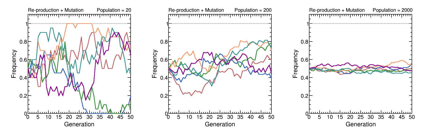
We can see there is no fixation or loss for a specific allele, because even if an allele is lost, it is still possible to appear again due to mutation. Therefore, genetic drift reduces the genetic diversity, while mutation increases the genetic diversity at the same time. They effect the dynamics of a population together. In next chapter, we will build a simple mathematical model to describe these two processes and discuss their roles under different configurations.
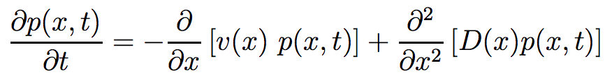
Let's consider a system with population size of N with a gene with two alleles (A1 and A2). To describe the frequency of one alleles, if there are n individuals with A1, we define x as the fraction of individuals with A1 in the whole population (x=n/N). A good variable to describe the whole system under random variation is probability density p(x,t), which means the probability of a population with A1 fraction of x at time t. p(x,t) satisfies the forward Kolmogorov equation
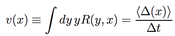
where v(x) is drift term, expressing the velocity with which transitions change:
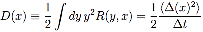
and D(x) is diffusion coefficient, characterizing the range of random variation of the probability function:
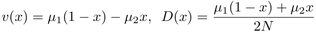
where R(y,x) is the rate of transition from state y to x. If the transition rate of A2 A1 (A1 A2) is μ1 (μ2), then
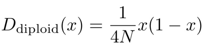
For genetic drift, if assuming no mutations (μ1=μ2=0), by employing binomial selection modelsee below, we can get for diploid,
Therefore, combining these two contributions, we can have the final drift and diffusion terms:

In terms of the forward Kolmogorov equation, it is interesting and technically easier to find the steady state solution to which the population settles after a long time, which is denoted as p*(x). Thus,
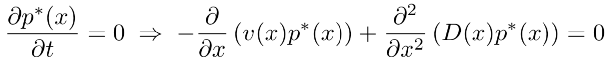
With v(x) and D(x) we find above, a steady probability density function under assumption μ1=μ2=μ as a function of x can be obtained:
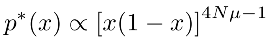
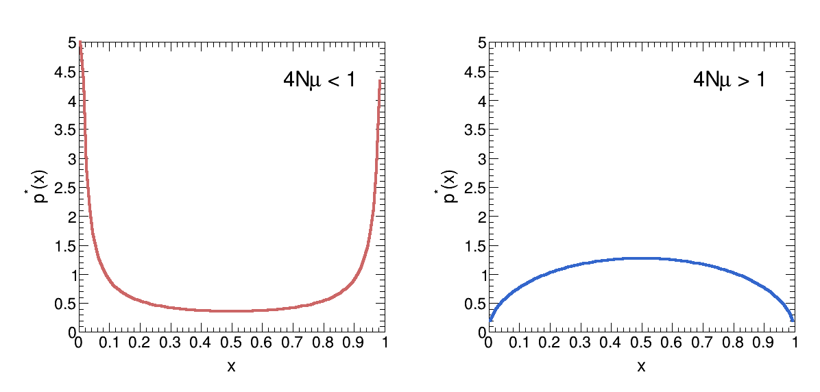
Therefore, the mutation scale is μ, and the genetic drift scale is 1/4N. When 4Nμ<1, the genetic drift is dominant, and therefore the system will reach fixation (loss) of an allele. When 4Nμ<1, the mutation is dominant, and therefore the system will reach an equilibrium at x=0.5.
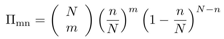
Consider a population of size N with two forms of an allele, A1 and A2. In the model of binomial selection, the new generation has the same size with the previous generation. Every individual has the same probability to produce a offspring. Therefore, if currently there are n individuals with A1, the probability to have m individuals in the next generation is